Poisson Distribution Enrichment

Scope Label

Enrichment / outside current 9758 core. This note is retained for comparison, teacher-directed extension, and coherence with some older teaching materials. Do not treat it as the main current core revision path unless instructed.

Use it with the hub Special Discrete Random Variables and the core branch Binomial Distribution.

What This Note Assumes

This note uses the same discrete-random-variable language as Discrete Random Variables:

• $X$ is the random variable
• $x$ is a possible non-negative integer value
• $P(X=x)$ is the probability of exactly $x$ occurrences

The new feature is the model structure: a Poisson variable counts occurrences over a stated interval or region. The interval is part of the model, not a decorative phrase.

The Poisson Situation

A Poisson random variable counts the number of random occurrences in a fixed interval.

The interval may be an interval of:

• time
• distance
• area
• volume
• page length
• any other measurable region

Examples include:

• number of phone calls in 10 minutes
• number of customers entering a shop in 5 minutes
• number of typing errors on a page
• number of accidents in a day
• number of particles emitted in a minute

If $X$ follows a Poisson distribution with mean $\lambda$, write:

$$X\sim \mathrm{Po}(\lambda ).$$

Here, $\lambda >0$ is the mean number of occurrences in the stated interval. (Allowing $\lambda =0$ gives only the degenerate count $X=0$.)

The phrase “in the stated interval” is essential. A Poisson mean belongs to a particular time or space interval.

A Poisson-process model is suitable when:

• occurrences are counted in an interval
• events occur randomly
• the mean count is proportional to interval size, corresponding to an approximately constant mean rate
• counts in disjoint intervals or regions are independent
• the probability of two or more occurrences in a sufficiently small interval is negligible

A Poisson variable has possible values:

$$0,1,2,3,\dots$$

Unlike a binomial variable, it has no fixed upper bound.

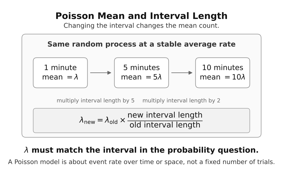How to read this enrichment figure. The symbol $\lambda$ in the first box is specifically the mean count in one minute. For the same stable process, five and ten times the interval length give means $5\lambda$ and $10\lambda$. The parameter is an interval mean, not a universal rate detached from its interval.

Understanding and Rescaling $\lambda$

For

$$X\sim \mathrm{Po}(\lambda ),$$

the parameter $\lambda$ means:

$$\lambda =\text{mean number of occurrences in the stated interval}.$$

It can help to separate the rate from the interval mean. If the mean rate is $\rho$ occurrences per unit time and the interval length is $t$, then

$$\lambda =\rho t.$$

This linear scaling assumes the same stable occurrence process across the interval. If a shop receives an average of 60 customers per hour, and $X$ is the number entering in one hour, then:

$$X\sim \mathrm{Po}(60).$$

But if $Y$ is the number entering in 5 minutes, the mean must be rescaled:

$$60\times \frac{5}{60}=5.$$

So:

$$Y\sim \mathrm{Po}(5).$$

In general, if the mean number of occurrences is $\lambda$ for an interval of length $T$, then the mean for an interval of length $t$ is:

$${\lambda }_{\text{new}}=\lambda \times \frac{t}{T}.$$

Always ask:

Does this $\lambda$ belong to the interval in the question?

Probability Function

For

$$X\sim \mathrm{Po}(\lambda ),$$

the probability of exactly $x$ occurrences is:

$$P(X=x)=e^{-\lambda }\frac{{\lambda }^x}{x!},x=0,1,2,\dots$$

The formula should not be used until $\lambda$ has been interpreted correctly.

Enrichment Example 1: Exact Poisson Probability

An average of 60 customers enter a store every hour. Find the probability that no customers enter during a particular 5-minute interval.

Let $X$ be the number of customers entering the store in 5 minutes.

The mean number in 5 minutes is:

$$60\times \frac{5}{60}=5.$$

Thus:

$$X\sim \mathrm{Po}(5).$$

We want:

$$P(X=0).$$

Using the Poisson formula:

$$P(X=0)=e^{-5}\frac{5^0}{0!}=e^{-5}.$$

Therefore:

$$P(X=0)\approx \mathrm{0.00674.}$$

The most important step is rescaling the mean from one hour to five minutes.

Mean, Variance, and Shape

For

$$X\sim \mathrm{Po}(\lambda ),$$

the mean is:

$$E(X)=\lambda .$$

The variance is:

$$\mathrm{Var}(X)=\lambda .$$

This equality is a characteristic consequence of the Poisson model:

$$E(X)=\mathrm{Var}(X).$$

This does not mean every data set with roughly equal mean and variance must be Poisson, nor does equality of mean and variance by itself define a distribution as Poisson.

The shape depends on $\lambda$:

• small $\lambda$ gives strong right skew
• larger $\lambda$ shifts the centre right
• larger $\lambda$ also increases spread
• the distribution becomes less strongly skewed as $\lambda$ increases

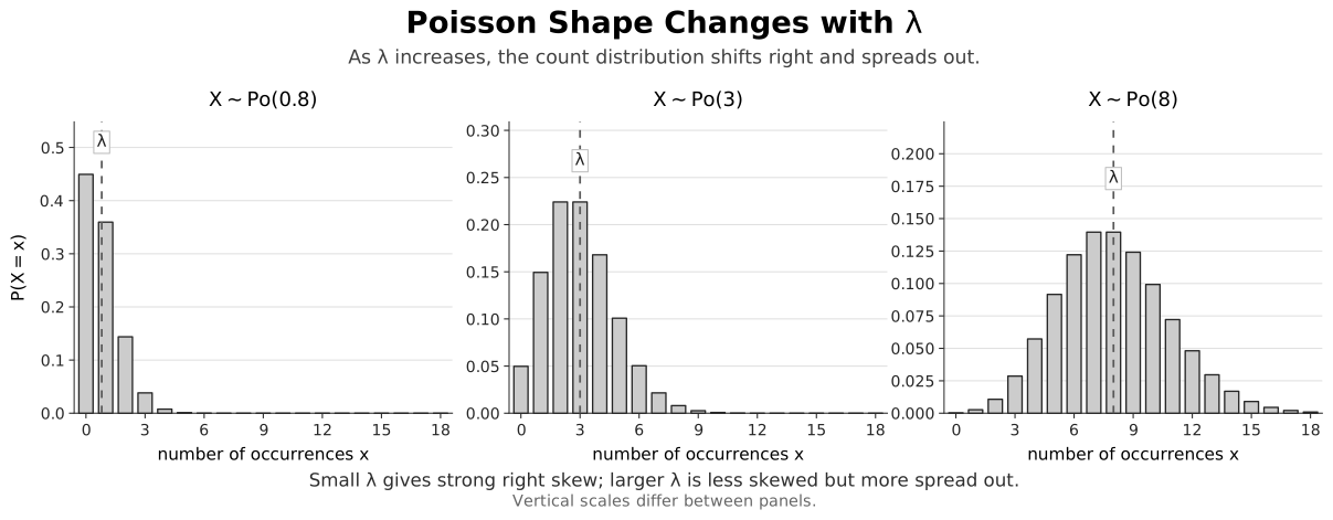How to read this enrichment figure. Each bar is a Poisson PMF mass. As $\lambda$ increases, both mean and variance increase, so the distribution moves right and spreads while becoming less skewed. The vertical scales differ between panels; compare location, spread, and skewness rather than raw bar heights across panels.

Cumulative Poisson Probabilities

The cumulative Poisson probability is:

$$P(X\le r).$$

For example, if $X\sim \mathrm{Po}(3.5)$, then:

$$P(X\ge 5)=1-P(X\le 4).$$

The same integer-valued translation discipline applies when $r$ is an integer:

Wording	Probability statement
at most $r$	$P(X\le r)$
fewer than $r$	$P(X\le r-1)$
at least $r$	$1-P(X\le r-1)$
more than $r$	$1-P(X\le r)$

Combining Independent Poisson Variables

Independent Poisson counts can be added by adding their means.

If

$$X\sim \mathrm{Po}({\lambda }_1),Y\sim \mathrm{Po}({\lambda }_2),$$

and $X$ and $Y$ are independent, then:

$$X+Y\sim \mathrm{Po}({\lambda }_1+{\lambda }_2).$$

This is useful when combining counts from independent sources or separate intervals.

For one Poisson process, counts in disjoint intervals are independent under the model. Overlapping intervals share occurrences and are therefore not independent. For different sources, independence must be justified by the context.

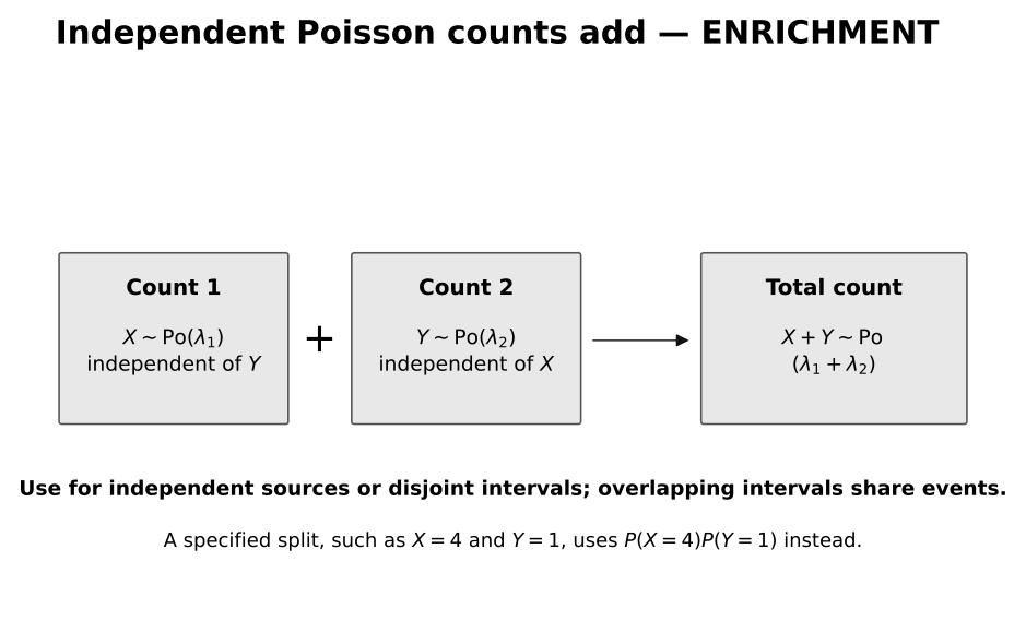
How to read this enrichment figure. Independent counts from disjoint intervals or independent sources add to a Poisson total whose mean is the sum of the component means. This total-count rule is different from asking for a specified split, which requires a joint probability.

Enrichment Example 2: Total Count Versus Specific Split

Suppose internal and external calls arrive independently at a switchboard.

Let:

$$X\sim \mathrm{Po}(3)$$

be the number of internal calls in 10 minutes, and:

$$Y\sim \mathrm{Po}(2)$$

be the number of external calls in 10 minutes.

For the total number of calls:

$$X+Y\sim \mathrm{Po}(5).$$

So the probability that a total of 5 calls arrive is:

$$P(X+Y=5).$$

Numerically,

$$P(X+Y=5)=e^{-5}\frac{5^5}{5!}\approx \mathrm{0.1755.}$$

But the probability of exactly 4 internal calls and exactly 1 external call is:

$$P(X=4\text{ and }Y=1)=P(X=4)P(Y=1),$$

because $X$ and $Y$ are independent.

Numerically,

$$P(X=4,Y=1)=\left(e^{-3}\frac{3^4}{4!}\right)\left(e^{-2}\frac{2^1}{1!}\right)\approx \mathrm{0.04548.}$$

This distinction matters:

• total count: add independent Poisson variables
• specific split: multiply probabilities for each independent part

Layered Poisson-Binomial Situations

Some enrichment questions use both Poisson and Binomial models.

For example, suppose the number of micro-organisms in one test-tube follows:

$$X\sim \mathrm{Po}(1.2).$$

The probability that a particular test-tube contains exactly 2 micro-organisms is:

$$q=P(X=2)=e^{-1.2}\frac{1.2^2}{2!}.$$

Now suppose 5 test-tubes are filled independently, and let $Y$ be the number of test-tubes that contain exactly 2 micro-organisms.

Each test-tube either:

• contains exactly 2 micro-organisms, with probability $q$
• does not contain exactly 2 micro-organisms, with probability $1-q$

So:

$$Y\sim B(5,q).$$

Here

$$q=e^{-1.2}\frac{1.2^2}{2!}\approx \mathrm{0.21686.}$$

For example, the probability that at least one of the five test-tubes contains exactly two micro-organisms is

$$P(Y\ge 1)=1-(1-q{)}^5\approx \mathrm{0.7054.}$$

The structure is:

1. use Poisson to find the probability of a property for one interval or item
2. use Binomial to count how many independent intervals or items have that property

Enrichment: Poisson Approximation to Binomial

Sometimes a binomial distribution can be approximated by a Poisson distribution.

If

$$X\sim B(n,p),$$

where $n$ is large and $p$ is small, then:

$$X\approx \mathrm{Po}(np).$$

Some older teaching materials give the following practical working guidelines:

• $n$ is large, often $n>50$
• $p$ is small, often $p<0.1$
• $np<5$

These are enrichment rules of thumb, not universal mathematical validity boundaries.

The conceptual reason is:

A large number of opportunities for a rare success begins to behave like a random rare-event count.

So we use:

$$\lambda =np.$$

Therefore:

$$B(n,p)\approx \mathrm{Po}(np).$$

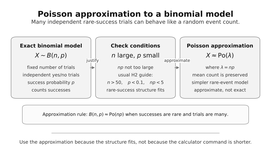How to read this enrichment figure. Begin with the exact Binomial mechanism, then justify a rare-success approximation and set $\lambda =np$. The displayed numerical cutoffs come from older practical guidance; they are not sharp boundaries between valid and invalid approximations.

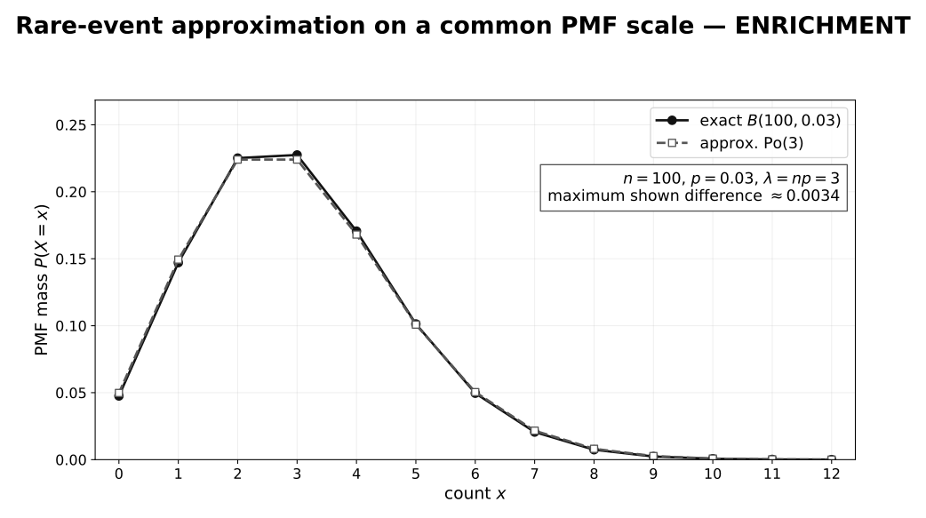
How to read this enrichment figure. The computed Binomial and Poisson PMFs use the same mean $np$. Their closeness in a valid rare-event example explains why the approximation can work; it remains an approximation, so a small probability error is expected.

Workflow for Poisson Approximation

A safe workflow is:

1. Start with the exact binomial model.
2. Check that $n$ is large and $p$ is small.
3. Compute $\lambda =np$.
4. Replace $B(n,p)$ by $\mathrm{Po}(np)$ approximately.
5. Translate the probability statement carefully.
6. Calculate using the Poisson model.

Do not apply a continuity correction when replacing a Binomial count by a Poisson count: both variables are discrete and use the same integer boundaries.

Do not begin by writing a Poisson model if the original situation is binomial. The approximation should be justified from the binomial model.

Enrichment Example 3: Rare Defects

Suppose 0.4% of peaches are rotten on arrival. A carton contains 250 individually packed peaches. Assuming independence, find approximately the probability that more than 3 peaches are rotten.

Let $X$ be the number of rotten peaches in the carton.

The exact model is:

$$X\sim B(250,0.004).$$

Here:

$$n=250,p=0.004,np=1.$$

Since $n$ is large, $p$ is small, and $np=1$, use:

$$X\approx \mathrm{Po}(1).$$

We want:

$$P(X>3)=1-P(X\le 3).$$

For $X\sim \mathrm{Po}(1)$:

$$P(X>3)=1-e^{-1}\left(1+1+\frac{1^2}{2!}+\frac{1^3}{3!}\right).$$

This gives approximately:

$$P(X>3)\approx \mathrm{0.0190.}$$

For comparison, direct evaluation of the exact Binomial tail gives

$$P_{B(250,0.004)}(X>3)\approx \mathrm{0.01874.}$$

The approximation error here is about $0.00025$. This comparison illustrates why the structural conditions matter and why “approximately” must be retained in the conclusion.

Common Pitfalls

Mistake	Better thinking
Treating $\lambda$ as a universal rate	$\lambda$ is the mean for a specific interval
Forgetting to rescale $\lambda$	Change the mean when the interval length changes
Treating every rare event as Poisson	Check the occurrence-process assumptions
Adding Poisson means without independence	The sum rule needs independent Poisson variables
Confusing total count with a specific split	Add variables for total count; multiply probabilities for a specified independent split
Using Poisson approximation without stating the Binomial model first	Begin with $X\sim B(n,p)$, then justify the approximation

Revision Checklist

• Can you explain what a Poisson random variable counts?
• Can you interpret $\lambda$ as an interval-specific mean?
• Can you rescale $\lambda$ when the interval changes?
• Can you calculate $P(X=x)$ and cumulative probabilities?
• Can you combine independent Poisson variables by adding their means?
• Can you distinguish total-count questions from specific-split questions?
• Can you identify when a Poisson approximation to Binomial is reasonable?
• Can you explain why this note is enrichment rather than current core revision?