Binomial Distribution

Scope Label

Core 9758. This branch is the main student-facing note for the current core special discrete model.

Use it with the hub Special Discrete Random Variables.

What This Note Assumes

This note assumes that you already know the general discrete-random-variable language from Discrete Random Variables.

In particular:

• $X$ is the random variable
• $r$ is one possible integer value of $X$
• $P(X=r)$ is the probability of the event that exactly $r$ successes occur

The Binomial distribution is a special case of this general language. It should only be used after the trial structure has been checked.

The Binomial Situation

A binomial random variable counts the number of successes in a fixed number of repeated trials.

A binomial model is appropriate when all of the following conditions are satisfied:

1. there is a fixed number $n$ of trials
2. each trial is classified into exactly two mutually exclusive and exhaustive categories, success and failure
3. the probability of success $p$ is the same for each trial
4. the trials are independent

If these conditions are satisfied, write:

$$X\sim B(n,p).$$

Here, $X$ counts the number of successes in the $n$ trials.

The word “success” does not necessarily mean something good. It simply means the classification being counted. A die has six raw outcomes, but “six” and “not six” form the two classifications needed for a binomial trial.

For example:

• if we count defective items, then “success” may mean “the item is defective”
• if we count sixes in die throws, then “success” means “a six is obtained”
• if we count correct answers in a guessed MCQ test, then “success” means “the answer is correct”

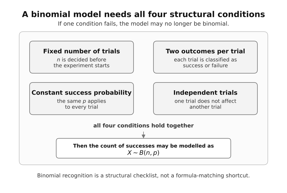How to read this figure. Check every box against the context: fixed $n$, success/failure classification, constant $p$, and independence. The arrow to $X\sim B(n,p)$ is justified only when all four hold together.

Checking the Conditions in Context

The four binomial conditions should be checked before calculation.

Condition	Meaning	Example
Fixed number of trials	The number of attempts is decided before the experiment starts.	A die is thrown 7 times.
Two classifications per trial	Every raw outcome belongs to exactly one of success or failure.	Six or not six.
Constant success probability	The value of $p$ does not change from trial to trial.	Each die throw has probability $\frac{1}{6}$ of giving a six.
Independence	One trial does not affect another trial.	One die throw does not affect the next.

If balls are drawn from a small finite bag without replacement, one result changes the composition available for later draws. The trials are then generally dependent and the success probability changes, so a binomial model is generally not exact.

A condition-failure counterexample

Suppose a bag contains 3 red and 2 blue balls and two balls are drawn without replacement. If “red” is success, the first-draw probability is $3/5$. After a red ball is drawn, the second-draw probability becomes $2/4$; after a blue ball, it becomes $3/4$. There is no single constant $p$, and the draws are not independent. Counting red balls here therefore requires direct sampling-without-replacement probability, not $B(2,3/5)$.

Stating the Random Variable and Distribution

A good solution should state the random variable clearly before using formulas.

A useful writing template is:

Let $X$ be the number of [successes] in [number of trials]. Then $X\sim B(n,p)$.

Example:

Let $X$ be the number of sixes obtained in 7 throws of a fair die. Then:

$$X\sim B\left(7,\frac{1}{6}\right).$$

Another example:

Let $Y$ be the number of correct answers obtained when a student guesses all 20 questions in a multiple-choice test with 4 options per question. Then:

$$Y\sim B\left(20,\frac{1}{4}\right).$$

This model statement confirms:

• what is being counted
• what one trial means
• what success means
• what $n$ is
• what $p$ is

Parameters and Possible Values

For

$$X\sim B(n,p),$$

• $n$ is the number of trials
• $p$ is the probability of success in each trial
• $1-p$ is the probability of failure in each trial
• $X$ is the number of successes

The possible values of $X$ are:

$$0,1,2,\dots ,n.$$

The parameter conditions are $n\in \{0,1,2,\dots \}$ and $0\le p\le 1$; in a non-empty repeated-trial context, $n$ is positive. An exact-value query uses an integer $r\in \{0,1,\dots ,n\}$.

This upper bound matters. A binomial random variable cannot exceed the number of trials.

For example, if

$$X\sim B\left(7,\frac{1}{6}\right),$$

then $P(X=8)$ is impossible because only 7 trials are performed.

Probability Function

For

$$X\sim B(n,p),$$

the probability of exactly $r$ successes is:

$$P(X=r)=\left(\genfrac{}{}{0ex}{}{n}{r}\right)p^r(1-p{)}^{n-r},r=0,1,2,\dots ,n.$$

The formula has a structure:

• $\left(\genfrac{}{}{0ex}{}{n}{r}\right)$ chooses the positions of the $r$ successes
• $p^r$ gives the probability of those successes
• $(1-p{)}^{n-r}$ gives the probability of the failures

So the formula is:

$$\text{number of success positions}\times \text{probability of one such pattern}.$$

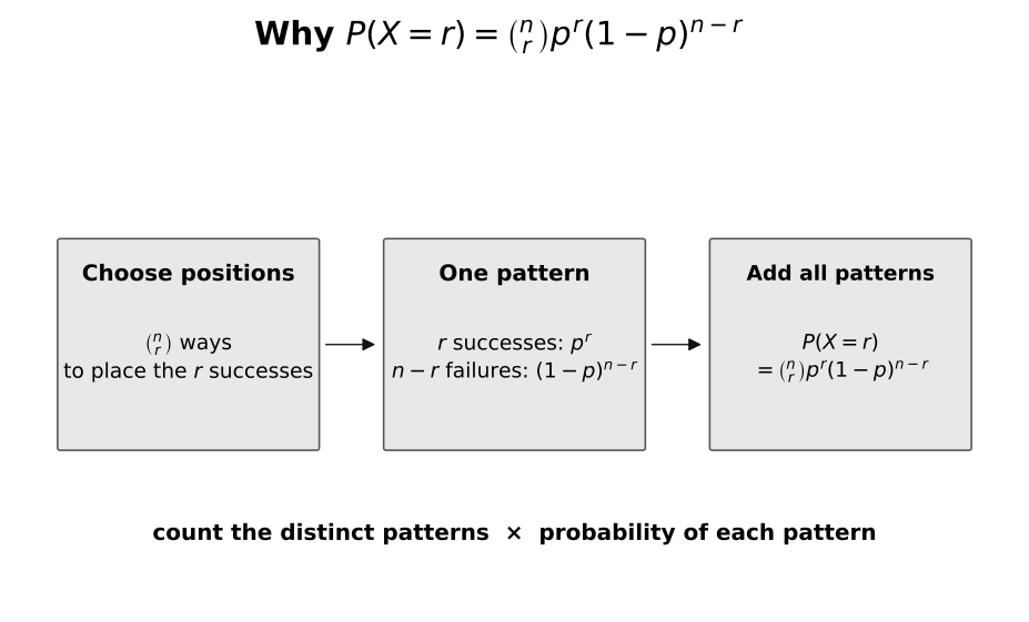
How to read this figure. For exactly $r$ successes, every particular success/failure pattern has probability $p^r(1-p{)}^{n-r}$. There are $\left(\genfrac{}{}{0ex}{}{n}{r}\right)$ different choices of the $r$ success positions, so multiplying these two factors gives the Binomial PMF.

Core Example 1: Exact Binomial Probability

A fair die is thrown 7 times. Find the probability of obtaining exactly 3 sixes.

Let $X$ be the number of sixes obtained in 7 throws.

Then:

$$X\sim B\left(7,\frac{1}{6}\right).$$

We want:

$$P(X=3).$$

Using the binomial formula:

$$P(X=3)=\left(\genfrac{}{}{0ex}{}{7}{3}\right){\left(\frac{1}{6}\right)}^3{\left(\frac{5}{6}\right)}^4.$$

This gives approximately:

$$P(X=3)\approx \mathrm{0.0781.}$$

The important modelling steps are:

1. define $X$
2. state $X\sim B(7,\frac{1}{6})$
3. translate the question into $P(X=3)$
4. calculate

Cumulative Binomial Probabilities

The cumulative binomial probability is:

$$P(X\le r).$$

It is useful for wording such as:

• at most $r$
• not more than $r$
• fewer than $r$
• at least $r$
• more than $r$

For integer-valued $X$ and integer threshold $r$:

Wording	Probability statement
exactly $r$	$P(X=r)$
at most $r$	$P(X\le r)$
fewer than $r$	$P(X<r)=P(X\le r-1)$
at least $r$	$P(X\ge r)=1-P(X\le r-1)$
more than $r$	$P(X>r)=1-P(X\le r)$

The difference between $X<r$ and $X\le r$ is one integer step.

Core Example 2: Cumulative Binomial Probability

Suppose

$$X\sim B(5,0.1).$$

Find $P(X\ge 2)$.

It is usually easier to use the complement:

$$P(X\ge 2)=1-P(X\le 1).$$

Since:

$$P(X\le 1)=P(X=0)+P(X=1),$$

we get:

$$P(X\ge 2)=1-\left[\left(\genfrac{}{}{0ex}{}{5}{0}\right)(0.9{)}^5+(\genfrac{}{}{0ex}{}{5}{1})(0.1)(0.9{)}^4\right].$$

This gives approximately:

$$P(X\ge 2)\approx \mathrm{0.0815.}$$

The key step is translating $X\ge 2$ as $1-P(X\le 1)$.

Core Example 2B: Probability Over an Inclusive Interval

If $X\sim B(12,0.3)$, find $P(3\le X\le 6)$.

For an integer-valued variable, the cumulative probability up to $6$ includes the unwanted values $0,1,2$. Hence

$$P(3\le X\le 6)=P(X\le 6)-P(X\le 2).$$

In CDF notation this is $F_X(6)-F_X(2)$. More generally, for integer $a\le b$,

$$P(a\le X\le b)=F_X(b)-F_X(a-1).$$

Evaluation gives

$$P(3\le X\le 6)\approx \mathrm{0.7086.}$$

The subtraction uses $a-1$, not $a$, because the lower endpoint $a$ must remain included.

Mean and Variance

For

$$X\sim B(n,p),$$

the mean is:

$$E(X)=np.$$

The variance is:

$$\mathrm{Var}(X)=np(1-p).$$

Why these formulas hold

Write the success count as

$$X=I_1+I_2+\cdots +I_n,$$

where $I_i=1$ if trial $i$ is a success and $I_i=0$ otherwise. Each Bernoulli indicator has

$$E(I_i)=p,\mathrm{Var}(I_i)=p(1-p).$$

Linearity of expectation gives

$$E(X)=\sum _{i=1}^{n}E(I_i)=np.$$

Because the trials—and therefore the indicators—are independent, their variances add:

$$\mathrm{Var}(X)=\sum _{i=1}^n\mathrm{Var}(I_i)=np(1-p).$$

The mean $np$ represents the expected number of successes.

For example, if a student guesses 20 multiple-choice questions with 4 options each, then:

$$X\sim B\left(20,\frac{1}{4}\right).$$

The expected number of correct answers is:

$$E(X)=20\left(\frac{1}{4}\right)=5.$$

The variance is:

$$\mathrm{Var}(X)=20\left(\frac{1}{4}\right)\left(\frac{3}{4}\right)=\frac{15}{4}.$$

The standard deviation is:

$$\sqrt{\frac{15}{4}}\approx \mathrm{1.94.}$$

Shape and Interpretation

A binomial distribution can be visualised using a probability histogram.

For fixed $n$:

• if $p$ is small, the distribution is skewed to the right
• if $p=0.5$, the distribution is symmetric
• if $p$ is large, the distribution is skewed to the left
• the centre of the distribution is near $np$

This is important because the binomial distribution is not just a formula. It is a full probability distribution with a shape.

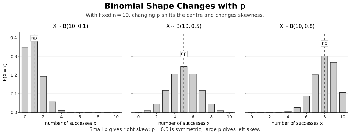How to read this figure. Each bar is a PMF mass $P(X=x)$. For fixed $n$, increasing $p$ moves the centre $np$ to the right and reverses the skew. The dashed line marks the mean $np$; a mean need not be an attainable integer or the most probable value.

Most Probable Value

The most probable value of a discrete random variable is the value with the largest probability.

It is the tallest bar in the probability histogram.

This value is not necessarily equal to $E(X)$.

For example, if

$$X\sim B\left(20,\frac{1}{4}\right),$$

then:

$$E(X)=5.$$

In this case, the most probable value is also $5$. But this agreement does not always happen.

To find the most probable value reliably, one may:

• inspect a probability table
• inspect a histogram
• compare neighbouring probabilities
• use calculator table values after the distribution has been correctly identified

A compact rule for $0<p<1$ is based on $(n+1)p$:

• if $(n+1)p$ is not an integer, the unique mode is $\lfloor (n+1)p\rfloor$
• if $(n+1)p=k$ is an integer, there are two adjacent modes, $k-1$ and $k$

At the boundary cases, $p=0$ gives mode $0$ and $p=1$ gives mode $n$.

Even when using this rule, a probability table or comparison of neighbouring PMF values is a useful check. The mean $np$ and the mode answer different questions.

Core Example 3: MCQ Guessing and Thresholds

A multiple-choice test has 20 questions with 4 options each. A student guesses all answers randomly.

Let $X$ be the number of correct answers.

Then:

$$X\sim B\left(20,\frac{1}{4}\right).$$

The mean is:

$$E(X)=20\left(\frac{1}{4}\right)=5.$$

The standard deviation is:

$$\sqrt{20\left(\frac{1}{4}\right)\left(\frac{3}{4}\right)}\approx \mathrm{1.94.}$$

Suppose we want the least value of $r$ such that:

$$P(X\le r)>\mathrm{0.85.}$$

Checking the cumulative probabilities gives:

$$P(X\le 6)\approx 0.78578,$$

while:

$$P(X\le 7)\approx \mathrm{0.89819.}$$

So the least value is:

$$r=7.$$

This example illustrates that cumulative probability questions often require a threshold search rather than one direct exact-value probability.

Combining Independent Binomial Samples

If two independent binomial counts have the same success probability, they can be combined. In general, if

$$X\sim B(m,p),Y\sim B(n,p),$$

and $X$ and $Y$ are independent, then

$$X+Y\sim B(m+n,p).$$

Both independence and the common value of $p$ matter. Independent binomial variables with different success probabilities do not generally have a binomial sum.

For example, suppose a sample of 10 items is drawn from a very large population where 10% of items are defective. Let $X$ be the number of defective items.

Then:

$$X\sim B(10,0.1).$$

If a second independent sample of 10 items is drawn under the same conditions, and $Y$ is its number of defectives, then:

$$Y\sim B(10,0.1).$$

The total number of defectives in the two samples is:

$$X+Y\sim B(20,0.1).$$

This works because the two samples together form 20 independent trials with the same success probability.

But be careful: if the question asks for a specific split, such as exactly one defective in each sample, then calculate the two sample events separately and multiply because of independence.

Calculator Workflow

A calculator is useful after the modelling has been done.

Use an exact-probability command for:

$$P(X=r).$$

Use a cumulative-probability command for:

$$P(X\le r).$$

Before using the calculator, write:

1. Let $X$ be the number of …
2. $X\sim B(n,p)$
3. Required probability $=...$

For an inclusive interval, use a CDF difference such as

$$P(a\le X\le b)=P(X\le b)-P(X\le a-1).$$

For an upper tail, use a complement. For a least/largest threshold, inspect adjacent cumulative values and report the pair that proves minimality or maximality, as in $F_X(6)\le 0.85<F_X(7)$.

The calculator should not replace model checking or probability-language translation.

For example, a calculator can evaluate $P(X\le r)$ quickly, but it cannot decide whether the problem should be modelled as $X\sim B(n,p)$ in the first place.

Common Pitfalls

Mistake	Better thinking
Forgetting that trials must be independent	Check whether one trial affects another
Forgetting that $p$ must remain constant	If the probability changes, the binomial model may fail
Confusing success with a desirable outcome	Success means the outcome being counted
Forgetting that $X$ only takes values $0,1,\dots ,n$	A binomial count cannot exceed the number of trials
Using $P(X\le r)$ when the question says $X<r$	For integer-valued $X$ and integer $r$, $X<r$ means $X\le r-1$
Starting with calculator commands	First define $X$, state the distribution, and translate the probability

Revision Checklist

• Can you state the four binomial conditions?
• Can you define success clearly in context?
• Can you write $X\sim B(n,p)$ with correct $n$ and $p$?
• Can you explain why the possible values are $0,1,\dots ,n$?
• Can you calculate $P(X=r)$?
• Can you use complements for “at least” and “more than” questions?
• Can you interpret $E(X)=np$ and $\mathrm{Var}(X)=np(1-p)$?
• Can you find a most probable value from a table or histogram?