Differentiation Techniques and Special Forms

Scope Label

Core 9758. This branch contains the main differentiation techniques, including implicit and parametric differentiation.

Use it with the hub Differentiation.

First Principles

First principles defines differentiation rather than merely giving rules.

For a curve $y=f(x)$, compare two nearby points:

$$(x,f(x))\text{and}(x+\delta x,f(x+\delta x)).$$

The chord gradient is

$$\frac{\delta y}{\delta x}=\frac{f(x+\delta x)-f(x)}{\delta x}.$$

Taking the limit as $\delta x\to 0$ gives the derivative:

$$f^{\prime }(x)=\underset{\delta x\to 0}{\lim }\frac{f(x+\delta x)-f(x)}{\delta x}.$$

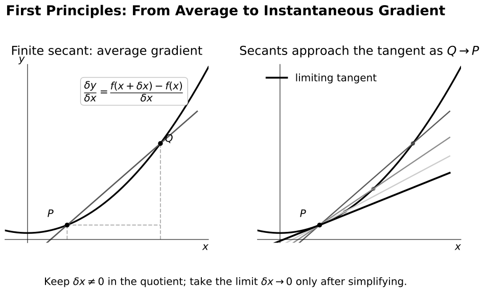How to read the figure. A secant gives an average rate of change. As its second point approaches the first, its gradient approaches the tangent gradient. Keep $\delta x\ne 0$ while simplifying the quotient; only then take the limit, provided that the limit exists.

You should understand:

• $\delta x$ as a small change in input;
• $\delta y$ as the corresponding change in output;
• $\frac{\delta y}{\delta x}$ as average rate of change;
• $f^{\prime }(x)$ as the limiting instantaneous rate of change.

Worked Example: First Principles

Find the derivative of

$$f(x)=x^2$$

from first principles.

Start with

$$f^{\prime }(x)=\underset{\delta x\to 0}{\lim }\frac{f(x+\delta x)-f(x)}{\delta x}.$$

Now

$$f(x+\delta x)=(x+\delta x{)}^2.$$

So

$$\frac{f(x+\delta x)-f(x)}{\delta x}=\frac{(x+\delta x{)}^2-x^2}{\delta x}.$$

Expand:

$$\frac{x^2+2x\delta x+(\delta x{)}^2-x^2}{\delta x}=2x+\delta x.$$

Therefore

$$f^{\prime }(x)=\underset{\delta x\to 0}{\lim }(2x+\delta x)=2x.$$

Standard Derivatives

The following results should be fluent:

Function	Derivative
$x^n$	$n{x}^{n-1}$
$\sin x$	$\cos x$
$\cos x$	$-\sin x$
$\tan x$	${\sec }^{2}x$
$e^x$	$e^x$
$\ln x$	$\frac{1}{x}$

Trigonometric derivative formulas assume radians. A fuller reference is:

Function	Derivative	Conditions
$a^x$	$a^x\ln a$	$a>0$
${\log }_{a}x$	$\frac{1}{x\ln a}$	$x>0$, $a>0$, $a\ne 1$
$\sec x$	$\sec x\tan x$	where $\sec x$ is defined
$\csc x$	$-\csc x\cot x$	where $\csc x$ is defined
$\cot x$	$-{\csc }^{2}x$	where $\cot x$ is defined

For an inner function $u=u(x)$, apply the chain factor $du/dx$. For example,

$$\frac{d}{dx}(\ln u)=\frac{1}{u}\frac{du}{dx}(u>0),\frac{d}{dx}(u^n)=n{u}^{n-1}\frac{du}{dx}$$

on intervals where the real-valued expressions and derivatives exist. The inverse-sine and inverse-cosine derivatives below are finite for $|x|<1$; the functions themselves also exist at the endpoints.

For composite forms, these are combined with the chain rule.

For example:

$$\frac{d}{dx}\sin (3x^2)=6x\cos (3x^2).$$

Inverse trigonometric derivatives may be treated as standard reference results when required by the question.

Common A-level inverse trigonometric results are:

Function	Derivative
${\sin }^{-1}x$	$\frac{1}{\sqrt{1-x^2}}$
${\cos }^{-1}x$	$-\frac{1}{\sqrt{1-x^2}}$
${\tan }^{-1}x$	$\frac{1}{1+x^2}$

For composite inputs, apply the chain rule. For example,

$$\frac{d}{dx}\left[{\tan }^{-1}(2x)\right]=\frac{2}{1+4x^2}.$$

Where both derivatives exist and neither is zero,

$$\frac{dx}{dy}=\frac{1}{\frac{dy}{dx}}.$$

This reciprocal relationship is useful, but it is not a licence to treat every derivative expression as an ordinary fraction without context. It works when $x$ can locally be treated as a differentiable function of $y$.

Chain Rule

Use the chain rule when one function is inside another.

If

$$y=f(g(x)),$$

then

$$\frac{dy}{dx}=f^{\prime }(g(x))g^{\prime }(x).$$

Example:

$$y=(3x^2+1{)}^5.$$

Then

$$\frac{dy}{dx}=5(3x^2+1{)}^4(6x).$$

So

$$\frac{dy}{dx}=30x(3x^2+1{)}^4.$$

The chain rule is the reason many special-looking techniques work.

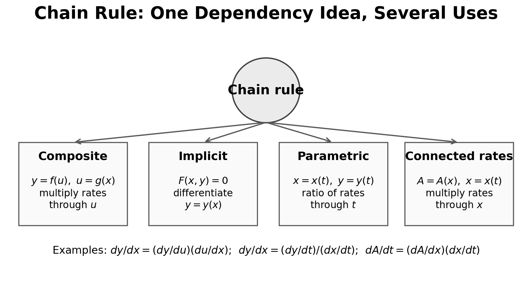How to read the figure. Begin with the required derivative and trace the intermediate dependency. Multiplication follows a chain of rates; parametric differentiation forms a ratio because both coordinates change through the same parameter.

Choosing and Combining Rules

Outermost structure	First choice
function inside a function	chain rule
product of changing factors	product rule
quotient of changing expressions	quotient rule
variable in both base and exponent, or a long product of powers	logarithmic differentiation
relation containing both $x$ and $y$	implicit differentiation
$x$ and $y$ given through a parameter	parametric differentiation

Rules often combine. If $y=x^2{e}^{3x}$, product rule acts first and chain rule differentiates $e^{3x}$:

$$\frac{dy}{dx}=2x{e}^{3x}+3x^2{e}^{3x}=x{e}^{3x}(2+3x).$$

Product and Quotient Rules

Use the product rule when two changing factors are multiplied:

$$\frac{d}{dx}(uv)=u\frac{dv}{dx}+v\frac{du}{dx}.$$

Use the quotient rule when one changing expression is divided by another:

$$\frac{d}{dx}\left(\frac{u}{v}\right)=\frac{v\frac{du}{dx}-u\frac{dv}{dx}}{v^2}.$$

The quotient formula applies where $v\ne 0$. The product and quotient rules should not be memorised as disconnected formulas. They respond to product and quotient structure.

For example,

$$\frac{d}{dx}[x^2\sin (3x)]=2x\sin (3x)+3x^2\cos (3x),$$

while, for $x\ne -1$,

$$\frac{d}{dx}\left(\frac{e^x}{x+1}\right)=\frac{(x+1)e^x-e^x}{(x+1{)}^2}=\frac{x{e}^x}{(x+1{)}^2}.$$

The second derivative means the derivative of the first derivative:

$$\frac{d^{2}y}{d{x}^2}=\frac{d}{dx}\left(\frac{dy}{dx}\right),$$

not ${\left(dy/dx\right)}^2$. It measures how gradient changes with $x$.

Logarithmic Differentiation

Logarithmic differentiation is useful when:

• the variable appears in both base and exponent, such as $y=x^x$;
• the expression is a complicated product or quotient of powers;
• taking logarithms simplifies the structure before differentiating.

Example:

$$y=x^x,x>0.$$

Take logarithms:

$$\ln y=x\ln x.$$

Differentiate implicitly:

$$\frac{1}{y}\frac{dy}{dx}=\ln x+1.$$

Hence

$$\frac{dy}{dx}=y(\ln x+1)=x^x(\ln x+1).$$

The key idea is not “take logs randomly”. Logs are useful because they turn powers and products into simpler differentiable structures.

Worked Example: Product of Powers

Differentiate

$$y=x^2\sqrt{x+1},x>0.$$

The restriction $x>0$ selects an interval on which every factor and $y$ are positive, so $\ln y$ is valid. The original algebraic function also exists for some non-positive $x$; those values would need a separate interval/sign analysis or the product-rule route. Logarithmic differentiation gives a cleaner structure on the stated interval:

$$\ln y=2\ln x+\frac{1}{2}\ln (x+1).$$

Differentiate:

$$\frac{1}{y}\frac{dy}{dx}=\frac{2}{x}+\frac{1}{2(x+1)}.$$

Thus

$$\frac{dy}{dx}=x^2\sqrt{x+1}\left(\frac{2}{x}+\frac{1}{2(x+1)}\right).$$

The final expression can be simplified if needed, but the main method is clear: logarithms turned a product of powers into a sum.

Implicit Differentiation

Use implicit differentiation when the curve is not given explicitly as $y=f(x)$.

For example:

$$x^2+y^2=25$$

does not express $y$ as one explicit function of $x$.

Differentiate both sides with respect to $x$:

$$2x+2y\frac{dy}{dx}=0.$$

So

$$\frac{dy}{dx}=-\frac{x}{y}.$$

The key discipline is:

$$\frac{d}{dx}[y]=\frac{dy}{dx},\frac{d}{dx}[y^2]=2y\frac{dy}{dx}.$$

You are differentiating with respect to $x$, but $y$ is itself changing with $x$.

Worked Example: Implicit Curve

Find $\frac{dy}{dx}$ for

$$x^2+y^2=4xy.$$

Differentiate both sides with respect to $x$:

$$2x+2y\frac{dy}{dx}=4\left(x\frac{dy}{dx}+y\right).$$

Collect the $\frac{dy}{dx}$ terms:

$$2y\frac{dy}{dx}-4x\frac{dy}{dx}=4y-2x.$$

So

$$\frac{dy}{dx}=\frac{4y-2x}{2y-4x}=\frac{2y-x}{y-2x}.$$

The important step is differentiating $xy$ by the product rule:

$$\frac{d}{dx}(xy)=x\frac{dy}{dx}+y.$$

The displayed quotient for $dy/dx$ is valid where $y-2x\ne 0$. If its denominator is zero, inspect the original curve and differentiated relation separately for a vertical tangent or singular point.

Second Derivative of an Implicit Curve

For $x^2+y^2=25$, the first derivative is $y^{\prime }=-x/y$. Differentiating again,

$$y^{\prime \prime }=-\frac{y-x{y}^{\prime }}{y^2}=-\frac{x^2+y^2}{y^3}=-\frac{25}{y^3},y\ne 0.$$

Parametric Differentiation

Sometimes a curve is described by a parameter $t$:

$$x=f(t),y=g(t).$$

As $t$ changes, both $x$ and $y$ change. The gradient of the curve is found by comparing their rates of change:

$$\frac{dy}{dx}=\frac{\frac{dy}{dt}}{\frac{dx}{dt}},\frac{dx}{dt}\ne 0.$$

Example:

$$x=t^2,y=t^3.$$

Then

$$\frac{dx}{dt}=2t,\frac{dy}{dt}=3t^2.$$

So

$$\frac{dy}{dx}=\frac{3t^2}{2t}=\frac{3t}{2},t\ne 0.$$

At $t=0$, both $dx/dt$ and $dy/dt$ vanish, so the ratio formula is unavailable. Here the limiting gradient $3t/2\to 0$ reveals a horizontal tangent at a singularly parametrised point; such exceptional values must be analysed rather than cancelled into the original formula.

The derivative is usually first found in terms of $t$. If needed, substitute back using the parametric equations.

For the second derivative,

$$\frac{d^{2}y}{d{x}^2}=\frac{\frac{d}{dt}\left(\frac{dy}{dx}\right)}{\frac{dx}{dt}},\frac{dx}{dt}\ne 0.$$

It is not $\frac{d^{2}y/d{t}^2}{d^{2}x/d{t}^2}$. If $dx/dt=0$, the ratio formula is unavailable; inspect the local curve, since the point may have a vertical tangent or be singular.

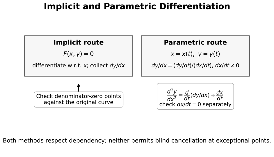
How to read the figure. The implicit route differentiates every term with respect to $x$ and collects $dy/dx$. The parametric route differentiates both coordinates with respect to $t$ and forms their ratio. The second-derivative route differentiates that ratio with respect to $t$ before dividing by $dx/dt$ again.

Worked Example: Tangent Gradient from a Parameter

Let

$$x=t^2+1,y=t^3-t.$$

Then

$$\frac{dx}{dt}=2t,\frac{dy}{dt}=3t^2-1.$$

Therefore

$$\frac{dy}{dx}=\frac{3t^2-1}{2t},t\ne 0.$$

Differentiate this gradient with respect to $t$:

$$\frac{d}{dt}\left(\frac{dy}{dx}\right)=\frac{d}{dt}\left(\frac{3t}{2}-\frac{1}{2t}\right)=\frac{3}{2}+\frac{1}{2t^2}.$$

Therefore

$$\frac{d^{2}y}{d{x}^2}=\left(\frac{3}{2}+\frac{1}{2t^2}\right)÷(2t)=\frac{3t^2+1}{4t^3},t\ne 0.$$

At $t=1$,

$$x=2,y=0,$$

and

$$\frac{dy}{dx}=1.$$

So the tangent at that point has equation

$$y=x-2.$$

This example shows why parametric differentiation belongs with tangents and normals: the parameter first gives the point, then the derivative gives the gradient.

How the Special Forms Are Related

The special forms are all ways of respecting how the curve or expression is built:

• explicit differentiation handles $y=f(x)$ directly;
• logarithmic differentiation simplifies powers/products first;
• implicit differentiation handles equations involving $x$ and $y$ together;
• parametric differentiation handles curves traced by a parameter.

The common principle is:

$$\text{identify structure first, then differentiate}.$$

Common Pitfalls

• Forgetting the chain rule on inner functions.
• Using the product rule where a chain rule is needed, or vice versa.
• Differentiating $y$ as if it were constant in implicit differentiation.
• Forgetting to multiply by $\frac{dy}{dx}$ when differentiating a function of $y$.
• For parametric curves, using $\frac{dy}{dt}$ as though it were $\frac{dy}{dx}$.
• Dividing by $\frac{dx}{dt}$ without noticing where it may be zero.
• Taking logarithms without checking that the expression is positive in the context.

Revision Checklist

• Can you identify the outermost structure before choosing a rule?
• Can you state domain and denominator restrictions?
• Can you distinguish $d^{2}y/d{x}^2$ from $(dy/dx{)}^2$?
• Can you differentiate an implicit relation and interpret exceptional points?
• Can you obtain both first and second parametric derivatives?

Related

• Differentiation
• Derivative Graph Behaviour and Applications
• Functions