Derivative Graph Behaviour and Applications

Scope Label

Core 9758. This branch develops the geometric and applied uses of derivatives: graph behaviour, tangents and normals, optimisation, and connected rates.

Use it with the hub Differentiation.

Increasing and Decreasing Functions

A function is strictly increasing on an interval if

$$x_1<x_2\Rightarrow f(x_1)<f(x_2)$$

for every $x_1,x_2$ in that interval. It is strictly decreasing if the final inequality is reversed. In this note, “increasing” and “decreasing” use these strict conventions unless stated otherwise.

The sign of the first derivative gives a convenient sufficient test for this behaviour.

If

$$f^{\prime }(x)>0$$

on an interval, then $f$ is increasing on that interval.

If

$$f^{\prime }(x)<0$$

on an interval, then $f$ is decreasing on that interval.

The phrase “on an interval” matters. Increasing and decreasing behaviour is not decided at one isolated point.

The conditions $f^{\prime }(x)>0$ or $f^{\prime }(x)<0$ throughout an interval are sufficient, but not always necessary, for strict monotonicity. For example, $f(x)=x^3$ is strictly increasing on $\mathbb{R}$ even though $f^{\prime }(0)=0$.

Stationary Points

A stationary point occurs when

$$f^{\prime }(x)=0.$$

At such a point, the tangent is horizontal.

A turning point is a point where the graph changes from increasing to decreasing or vice versa. A point of inflexion is a point across which concavity changes. Therefore a stationary point need not turn, and an inflexion need not be stationary.

Common examinable stationary-point behaviours are:

• local maximum;
• local minimum;
• stationary point of inflexion.

A stationary point is a candidate for a turning point, but it is not automatically a maximum or minimum.

Classifying Stationary Points

First Derivative Test

Check the sign of $f^{\prime }(x)$ just before and just after the stationary point.

Signs of $f^{\prime }(x)$ on the left and right	Nature
$+$ to $-$	local maximum
$-$ to $+$	local minimum
$+$ to $+$	no turning point; test concavity to decide whether there is an inflexion
$-$ to $-$	no turning point; test concavity to decide whether there is an inflexion

This test is often the most reliable because it directly checks whether the graph turns.

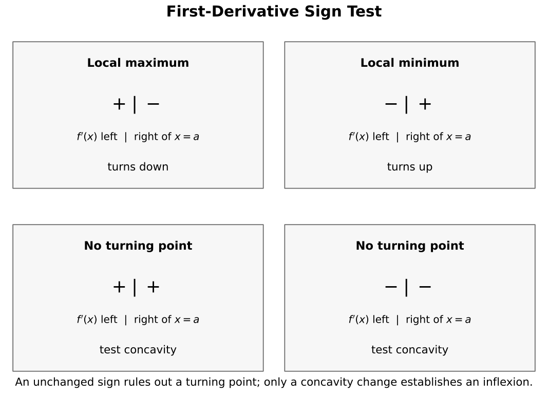How to read the figure. Read each sign line from left to right. A $+\to -$ change means increasing then decreasing, hence a local maximum; $-\to +$ gives a local minimum. An unchanged sign proves only that there is no turning point. It does not by itself prove an inflexion: concavity must also change.

Second Derivative Test

At a stationary point:

• if $f^{\prime \prime }(x)<0$, the point is a local maximum;
• if $f^{\prime \prime }(x)>0$, the point is a local minimum;
• if $f^{\prime \prime }(x)=0$, the test is inconclusive.

The test works by tracking the gradient through zero. If $f^{\prime \prime }(a)>0$, gradients increase from negative to positive around the stationary point, so the graph turns upwards and has a local minimum. If $f^{\prime \prime }(a)<0$, gradients decrease from positive to negative, giving a local maximum. These conclusions require $f^{\prime }(a)=0$ and the relevant derivatives to exist around the point.

If $f^{\prime \prime }(a)$ does not exist, the second-derivative test cannot be applied; use the first-derivative sign test or direct graph behaviour.

When the second derivative test is inconclusive, return to the first derivative test or inspect the graph behaviour directly.

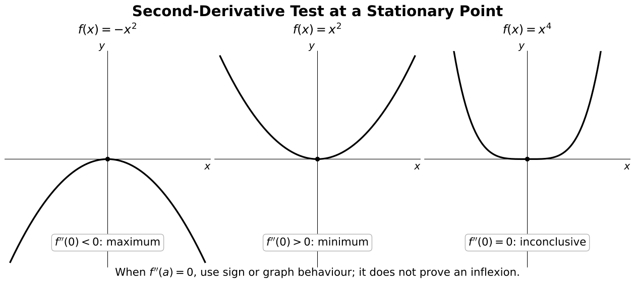
How to read the figure. The first two panels show the conclusive cases at a stationary point: negative second derivative gives a local maximum and positive second derivative gives a local minimum. The $x^4$ panel is the warning case: $f^{\prime \prime }(0)=0$ even though the point is a minimum, so the first-derivative sign test is still required.

Example:

$$f(x)=x^4$$

has

$$f^{\prime }(x)=4x^3,f^{\prime \prime }(x)=12x^2.$$

At $x=0$,

$$f^{\prime }(0)=0,f^{\prime \prime }(0)=0.$$

The second derivative test is inconclusive. But $f^{\prime }(x)<0$ for $x<0$ and $f^{\prime }(x)>0$ for $x>0$, so the graph changes from decreasing to increasing. Hence $x=0$ gives a local minimum.

Local Versus Global Extrema

A local maximum or minimum is only compared with nearby points.

A global maximum or minimum is compared across the whole relevant domain.

This distinction matters in application questions. Endpoints, restrictions, and physical context may determine the true maximum or minimum even when stationary points exist.

Concavity

The second derivative describes how the gradient changes.

• if $f^{\prime \prime }(x)>0$ on an interval, the graph is concave upwards there;
• if $f^{\prime \prime }(x)<0$ on an interval, the graph is concave downwards there.

The correct reasoning chain is:

• $f^{\prime \prime }(x)$ tells you how $f^{\prime }(x)$ changes;
• if $f^{\prime }(x)$ is increasing, the curve is concave upwards;
• if $f^{\prime }(x)$ is decreasing, the curve is concave downwards.

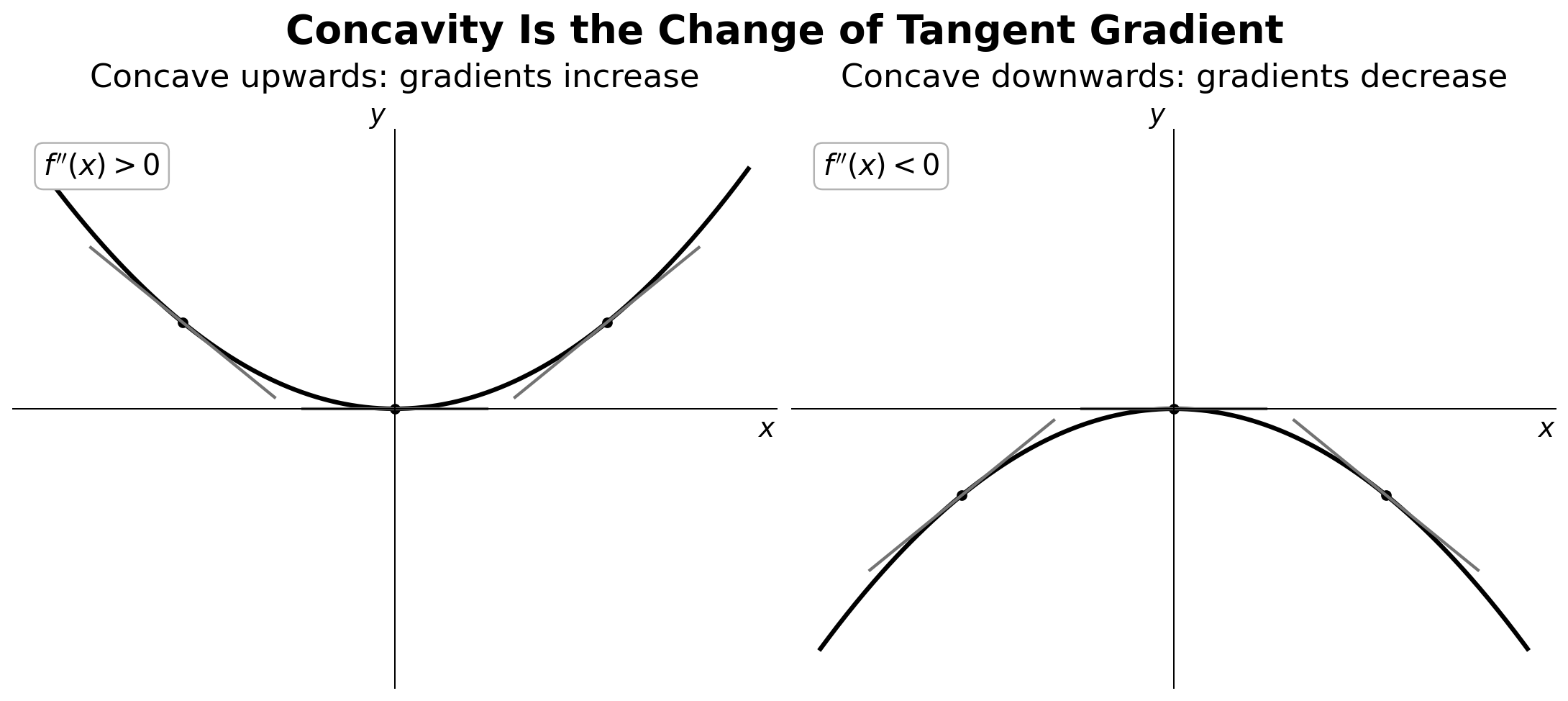How to read the figure. Compare tangent gradients as $x$ increases. On a concave-up interval they become larger; on a concave-down interval they become smaller. This remains true whether the curve lies above or below the $x$-axis.

The equation $f^{\prime \prime }(a)=0$ only identifies a possible inflexion for a sufficiently smooth curve. Verify that $f^{\prime \prime }$ changes sign, or otherwise show that concavity changes. An inflexion need not be stationary: $f(x)=x^3+x$ has an inflexion at $x=0$ but $f^{\prime }(0)=1$.

Worked Example: Concavity Intervals

For

$$f(x)=x^3-3x,$$

the domain is all real numbers and

$$f^{\prime \prime }(x)=6x.$$

Thus $f^{\prime \prime }(x)<0$ for $x<0$, so the graph is concave downwards on $(-\infty ,0)$. Also $f^{\prime \prime }(x)>0$ for $x>0$, so it is concave upwards on $(0,\infty )$. The second derivative changes sign at $x=0$, and $f(0)=0$, so $(0,0)$ is a point of inflexion. There are no excluded domain boundaries to test in this example.

Graph of the Derivative Function

The graph of $y=f^{\prime }(x)$ records gradient information about $y=f(x)$.

Key links:

• zeros of $f^{\prime }(x)$ match stationary points of $f$;
• $f^{\prime }(x)>0$ means $f$ is increasing;
• $f^{\prime }(x)<0$ means $f$ is decreasing;
• turning points of $f^{\prime }(x)$ may correspond to changes in concavity of $f$.

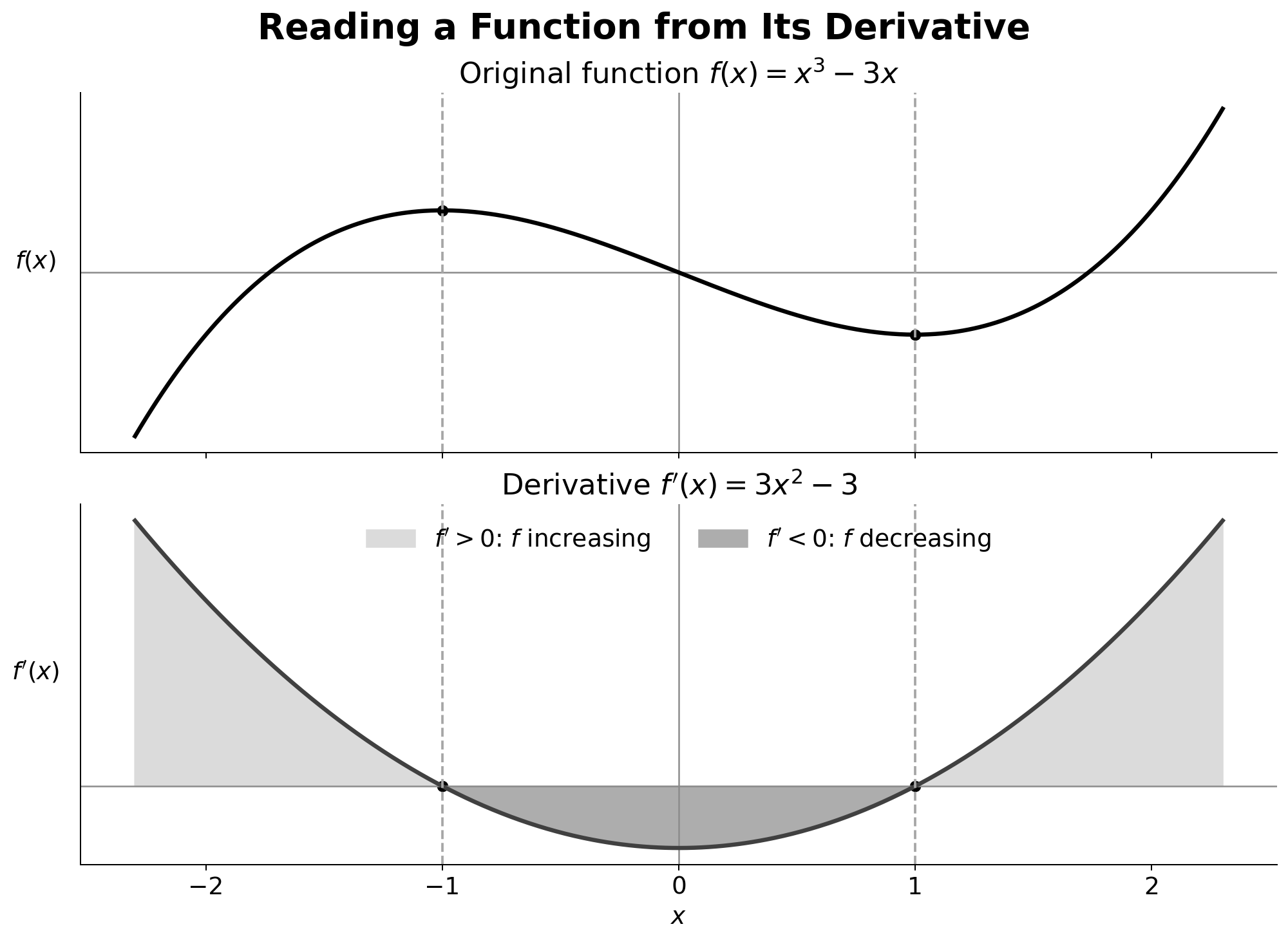How to read the figure. Align the same $x$-coordinate in both panels. Zeros of $f^{\prime }$ locate horizontal tangents of $f$, while the sign of $f^{\prime }$ tells whether $f$ rises or falls. A turning point of $f^{\prime }$ can indicate a possible inflexion of $f$, but verify the associated change in concavity.

Tangents and Normals

At a point $(a,b)$ on a curve, the tangent has the same direction as the curve at that point.

If the curve is $y=f(x)$ and $b=f(a)$, then the tangent gradient is

$$m=f^{\prime }(a).$$

The tangent equation is

$$y-b=m(x-a).$$

The normal is perpendicular to the tangent. If the tangent gradient is $m\ne 0$, then the normal gradient is

$$-\frac{1}{m}.$$

So the normal equation is

$$y-b=-\frac{1}{m}(x-a).$$

Special cases:

• if $m=0$, the tangent is horizontal and the normal is vertical;
• if the tangent is vertical, the usual finite-gradient formula does not apply.

These ideas apply to explicit, implicit, and parametric curves. The main difference is how you obtain the tangent gradient.

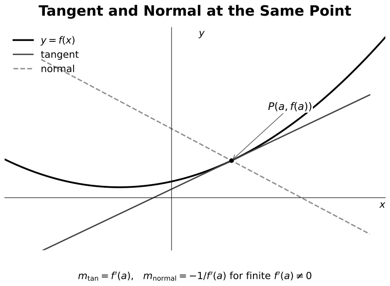How to read the figure. The tangent and normal meet at the stated point on the curve. For a finite non-zero tangent gradient $m$, the normal gradient is $-1/m$. If the tangent is horizontal, the normal is the vertical line $x=a$; if the tangent is vertical, the normal is the horizontal line $y=b$.

Worked Example: Tangent and Normal

For the curve

$$y=(x-1{)}^2$$

at $x=2$, the point is

$$(2,1).$$

The derivative is

$$\frac{dy}{dx}=2(x-1),$$

so the tangent gradient at $x=2$ is

$$m=2.$$

The tangent is

$$y-1=2(x-2).$$

The normal gradient is

$$-\frac{1}{2},$$

so the normal is

$$y-1=-\frac{1}{2}(x-2).$$

Optimisation

Maxima and minima problems ask you to optimise a quantity under constraints.

A reliable workflow is:

1. identify the quantity to maximise or minimise;
2. express it as a function of one variable;
3. state the domain or contextual restrictions;
4. differentiate;
5. find stationary values;
6. test whether each stationary value gives a maximum or minimum;
7. compare with endpoints or contextual restrictions where necessary;
8. answer in context.

The stationary-value step is only part of the argument. A fluent derivative calculation can still give the wrong answer if the model or domain is wrong.

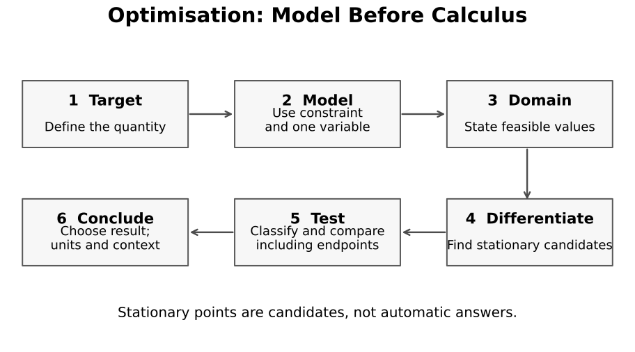How to read the figure. Calculus begins only after the target, constraint and feasible domain are defined. Solving $Q^{\prime }(x)=0$ produces interior candidates, not an automatic answer. Compare all valid candidates and required endpoints before interpreting the optimum with units.

Worked Example: Fixed Sum, Maximum Area

A right-angled triangle has perpendicular sides $x$ and $10-x$. Its area is

$$A=\frac{1}{2}x(10-x)=5x-\frac{1}{2}{x}^2.$$

Differentiate:

$$\frac{dA}{dx}=5-x.$$

Set

$$\frac{dA}{dx}=0$$

to get

$$x=5.$$

Since

$$\frac{d^{2}A}{d{x}^2}=-1<0,$$

this gives a maximum. The maximum area is

$$A=\frac{1}{2}(5)(5)=\mathrm{12.5.}$$

The physical domain is $0<x<10$. The area tends to $0$ at the degenerate endpoint cases, and the only interior stationary point gives $12.5$. Hence this stationary value is the global maximum over the feasible range.

The derivative step is short; the main modelling step is expressing the area as a one-variable function.

Worked Example: Eliminate a Constraint Variable

A closed cylinder has fixed volume $V>0$. With radius $r>0$ and height $h$,

$$\pi r^{2}h=V\Rightarrow h=\frac{V}{\pi r^2}.$$

Its surface area becomes the one-variable function

$$S=2\pi r^2+2\pi rh=2\pi r^2+\frac{2V}{r},r>0.$$

Hence

$$\frac{dS}{dr}=4\pi r-\frac{2V}{r^2}.$$

At a stationary value,

$$4\pi r^3=2V\Rightarrow r={\left(\frac{V}{2\pi }\right)}^{1/3}.$$

Moreover,

$$\frac{d^{2}S}{d{r}^2}=4\pi +\frac{4V}{r^3}>0.$$

Since $S\to \infty$ as $r\to 0^{+}$ and as $r\to \infty$, this stationary value gives the global minimum. The key modelling move was using the volume constraint to eliminate $h$ before differentiating.

Connected Rates

Connected-rates problems involve two or more quantities changing with time.

The chain rule is the main idea.

If $A=f(x)$ and $x$ changes with time $t$, then

$$\frac{dA}{dt}=\frac{dA}{dx}\frac{dx}{dt}.$$

In this explicit case, $\frac{dA}{dx}$ comes from the relationship between the variables, while $\frac{dx}{dt}$ is the known time-rate. For an implicit relationship, differentiate the whole equation with respect to $t$.

The safe workflow is:

1. write a relationship between the variables;
2. differentiate with respect to time;
3. substitute the values relevant to the instant;
4. solve for the required rate;
5. interpret the sign.

Do not substitute instant-specific values before differentiating unless the value is a constant for all time.

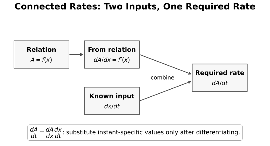How to read the figure. The relation supplies a conversion between rates. Differentiate the general relation first, then insert values for the stated instant. Preserve signs and units: a negative result means the required quantity is decreasing.

Worked Example: Connected Rates

For a ladder of fixed length $5$ m leaning against a wall, let the base distance be $x$ and the height be $h$.

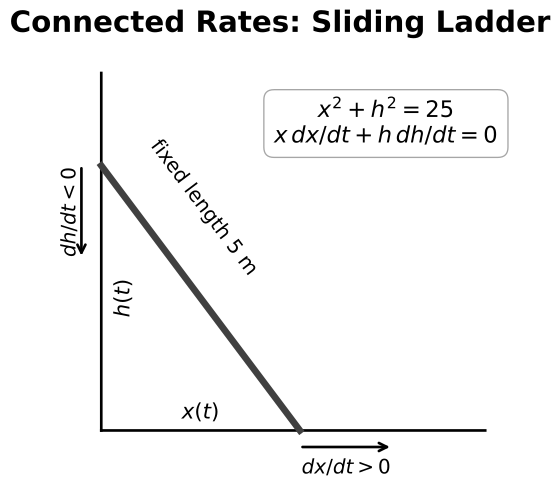
How to read the figure. The ladder length is fixed, so $x$ and $h$ are linked by Pythagoras. The rightward base arrow means $dx/dt>0$, while the downward top arrow anticipates $dh/dt<0$. Differentiating the geometric relation converts the known horizontal rate into the required vertical rate.

Then

$$x^2+h^2=25.$$

Differentiate with respect to time $t$:

$$2x\frac{dx}{dt}+2h\frac{dh}{dt}=0.$$

Suppose the base moves away from the wall at $0.4\mathrm{m}{\mathrm{s}}^{-1}$ when $x=3$ m. The relation gives $h=4$ m. Substituting only after differentiating,

$$2(3)(0.4)+2(4)\frac{dh}{dt}=0,$$

so

$$\frac{dh}{dt}=-0.3\mathrm{m}{\mathrm{s}}^{-1}.$$

Thus the top of the ladder is moving downwards at $0.3\mathrm{m}{\mathrm{s}}^{-1}$. The sign, unit and direction all belong to the answer.

Worked Example: Rates with Area and Volume

A spherical balloon has radius $r$, surface area $A=4\pi r^2$, and volume $V=\frac{4}{3}\pi r^3$. When $r=10$ cm, its surface area increases at $6.4\mathrm{c}{\mathrm{m}}^2{\mathrm{s}}^{-1}$.

First,

$$\frac{dA}{dt}=8\pi r\frac{dr}{dt},$$

so at the stated instant,

$$\frac{dr}{dt}=\frac{6.4}{80\pi }\approx 0.0255\mathrm{cm}{\mathrm{s}}^{-1}.$$

Then

$$\frac{dV}{dt}=4\pi r^2\frac{dr}{dt}=4\pi (10{)}^2\left(\frac{6.4}{80\pi }\right)=32\mathrm{c}{\mathrm{m}}^3{\mathrm{s}}^{-1}.$$

This example shows why units change with the quantity: radius, area and volume rates have units of length, area and volume per unit time respectively.

Revision Checklist

• Can you distinguish stationary, turning and inflexion points?
• Can you classify a stationary point without assuming that $f^{\prime \prime }=0$ proves anything?
• Can you map signs and zeros of $f^{\prime }$ back to the behaviour of $f$?
• Can you handle horizontal and vertical tangent/normal cases?
• Can you define an optimisation domain and compare all candidates?
• Can you keep units and interpret the sign in a connected-rates result?

Common Pitfalls

• Assuming $f^{\prime }(x)=0$ automatically means a maximum or minimum.
• Using the second derivative test when it is inconclusive, without checking signs of $f^{\prime }(x)$.
• Confusing a local extremum with a global extremum.
• Confusing concavity with increasing or decreasing behaviour.
• Using a tangent or normal formula with a point that is not on the curve.
• Forgetting vertical or horizontal tangent/normal special cases.
• In connected-rates problems, substituting instant-specific values before differentiating.
• Giving a rate without interpreting whether it is increasing or decreasing.

Related

• Differentiation
• Differentiation Techniques and Special Forms
• Functions