First-Order Separable and Modelling

Scope Label

Core 9758. This is the main examinable route for differential equations: first-order separable equations and simple modelling from rate statements.

Use this branch with the hub Differential Equations.

The Structural Question

For a first-order differential equation, the key question is:

$$\frac{dy}{dx}\text{depends on what?}$$

The common core forms are:

• $\frac{dy}{dx}=f(x)$;
• $\frac{dy}{dx}=g(y)$;
• $\frac{dy}{dx}=f(x)g(y)$.

These are not arbitrary categories. They tell you how the derivative can be undone.

Form 1: Direct Integration

If

$$\frac{dy}{dx}=f(x),$$

then solve by integrating with respect to $x$:

$$y=\int f(x)dx+C.$$

Example:

$$\frac{dy}{dx}=3x^2-4$$

gives

$$y=x^3-4x+C.$$

This is still a differential-equation solution, even though the method looks like ordinary integration.

Form 2: Depends Only on $y$

If

$$\frac{dy}{dx}=g(y),$$

first check any roots of $g(y)=0$. They may be constant equilibrium solutions. For non-equilibrium branches, work on intervals where $g(y)\ne 0$ and separate:

$$\frac{1}{g(y)}dy=dx.$$

Integrate both sides:

$$\int \frac{1}{g(y)}dy=\int dx.$$

Conceptually, the rate of change is controlled by the current value of $y$. This is why equations of this kind often appear in growth, decay, cooling, and evaporation models.

Form 3: Variables Separable

If

$$\frac{dy}{dx}=f(x)g(y),$$

first check $g(y)=0$ for constant solutions. Then, on intervals where $g(y)\ne 0$, rearrange to put all $y$-dependence on one side and all $x$-dependence on the other:

$$\frac{1}{g(y)}dy=f(x)dx.$$

Then integrate:

$$\int \frac{1}{g(y)}dy=\int f(x)dx.$$

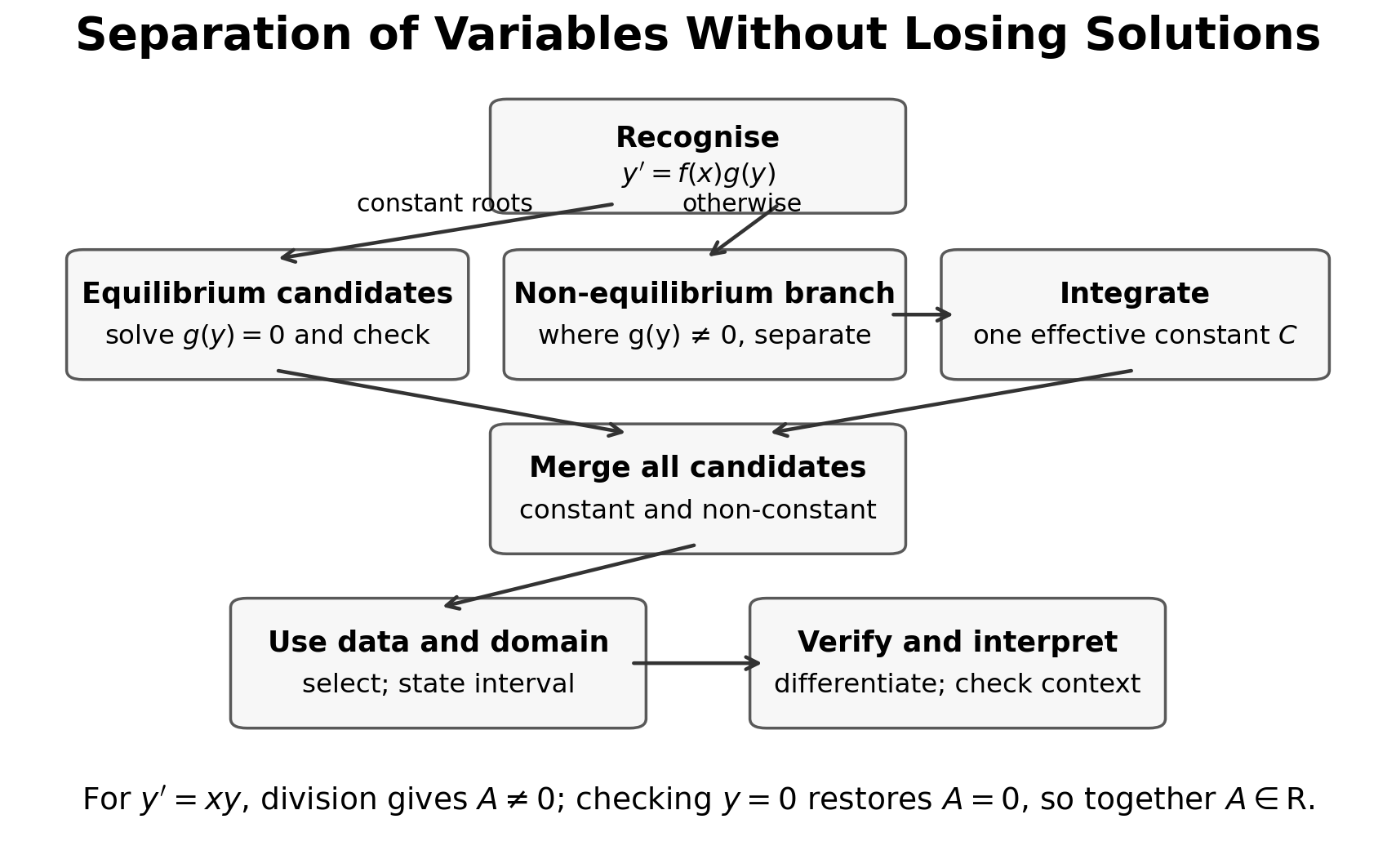How to read the figure. The first branch checks $g(y)=0$, because division could otherwise lose equilibrium solutions. The non-equilibrium branch separates variables, integrates with one effective arbitrary constant, applies data, states the interval, and verifies the result.

Worked Example: Variables Separable

Solve

$$\frac{dy}{dx}=xy.$$

First, $y=0$ satisfies the original equation. For a non-zero solution, separate variables:

$$\frac{1}{y}dy=xdx.$$

Integrate:

$$\int \frac{1}{y}dy=\int xdx.$$

Thus

$$\ln |y|=\frac{x^2}{2}+C.$$

Exponentiating gives

$$|y|=e^C{e}^{x^2/2}.$$

Absorbing the sign and $e^C$ into a non-zero constant $A$ gives the non-zero family. Restoring the checked equilibrium solution allows us to write the complete family compactly as

$$y=A{e}^{x^2/2},A\in \mathbb{R}.$$

The arbitrary constant may be renamed. For example, the accompanying figure writes the same family as $y=C_1{e}^{x^2/2}$.

For the non-zero branch, it is acceptable to leave the answer implicitly as

$$\ln |y|=\frac{x^2}{2}+C,$$

unless the question asks for $y$ explicitly. This logarithmic form excludes $y=0$; the complete solution set is expressed most compactly by $y=A{e}^{x^2/2}$ with $A\in \mathbb{R}$.

Separable Variants

Separable equations appear in several common variants. They look different, but the structural question is the same:

Can all $y$-dependence be moved to one side and all $x$-dependence to the other?

Variant 1: derivative depends only on $y$

Solve

$$\frac{dy}{dx}=1+y^2.$$

Since the right-hand side depends only on $y$, separate variables:

$$\frac{1}{1+y^2}dy=dx.$$

Integrate:

$${\tan }^{-1}y=x+C.$$

This is a valid implicit general solution. If required,

$$y=\tan (x+C).$$

Each solution is defined only on an interval that avoids the vertical asymptotes, where $x+C\ne \frac{\pi }{2}+n\pi$.

The important point is that the integration is with respect to $y$ on the left and with respect to $x$ on the right.

Variant 2: exponential dependence on $y$

Solve

$$\frac{dy}{dx}=2e^y.$$

Separate variables:

$$e^{-y}dy=2dx.$$

Integrate:

$$-e^{-y}=2x+C.$$

Equivalently,

$$e^{-y}=A-2x,$$

where $A$ is an arbitrary constant.

This example is useful because it reminds you that solving explicitly for $y$ is not always necessary unless the question asks for it. If solving explicitly,

$$y=-\ln (A-2x),$$

on intervals where $A-2x>0$.

Variant 3: product of an $x$-part and a $y$-part

Solve

$$\frac{dy}{dx}=(x-3)y.$$

Separate variables:

$$\frac{1}{y}dy=(x-3)dx.$$

Integrate:

$$\ln |y|=\frac{x^2}{2}-3x+C.$$

Therefore,

$$y=A{e}^{x^2/2-3x},$$

with the usual caution that division by $y$ has separated out the non-zero family; $y=0$ is also a solution of the original differential equation.

Algebra Discipline

Separation of variables is not a decorative rewriting trick. Each step must be justified by multiplication or division.

For example, from

$$\frac{dy}{dx}=xy,$$

we divide by $y$ and multiply by $dx$.

The warning is that division can lose possible solutions. In the example above, $y=0$ is also a solution of $\frac{dy}{dx}=xy$. Some school-level solutions focus on the non-zero family; a careful solution should at least notice whether division by a variable expression may exclude a solution.

Practical rules:

• move $y$-dependent factors by legitimate algebraic steps;
• avoid dividing by a quantity without noticing whether it could be zero;
• include the arbitrary constant after integrating;
• apply initial conditions only after obtaining the general solution.

Initial Conditions

A general solution contains arbitrary constants. An initial condition selects one particular solution.

Example:

$$\frac{dy}{dx}=xy,y(0)=3.$$

From the previous example,

$$y=A{e}^{x^2/2}.$$

Use $y(0)=3$:

$$3=A{e}^0,$$

so

$$A=3.$$

The particular solution is

$$y=3e^{x^2/2}.$$

Modelling from Rate Statements

A modelling question asks you to translate language about change into a differential equation.

The usual chain is:

$$\text{words}⟶\text{rate statement}⟶\text{differential equation}.$$

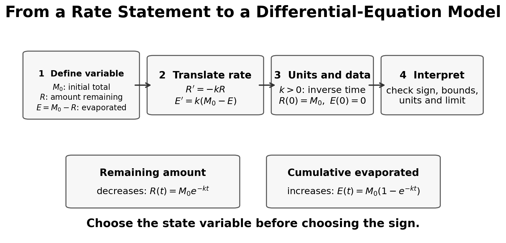How to read the figure. Follow the modelling chain from the wording to a clearly defined state variable, the derivative sign, the constant $k$ and its units, and then the initial condition and solution. The adjacent evaporation example shows why choosing cumulative amount instead of remaining amount reverses the sign convention.

Common Language Cues

Phrase	Typical interpretation
rate of change of $y$	$\frac{dy}{dx}$ or $\frac{dy}{dt}$
rate of increase	positive derivative
quantity decreases	its derivative is negative
rate of decrease stated as a positive magnitude	$-\frac{dx}{dt}$ equals that positive rate
proportional to	equals a constant times
amount remaining	total amount minus amount used, lost, or evaporated

For example:

The rate of decrease of a quantity $x$ is proportional to the amount remaining.

If $x$ is the amount remaining, then

$$\frac{dx}{dt}=-kx,k>0.$$

The negative sign records the decrease.

Growth and Decay

The two most common patterns are:

$$\frac{dx}{dt}=kx\text{growth}$$

and

$$\frac{dx}{dt}=-kx\text{decay},$$

where $k>0$. If $t$ is measured in seconds, $k$ has unit ${\mathrm{s}}^{-1}$; in general its unit is inverse time.

For decay,

$$\frac{dx}{dt}=-kx$$

separates as

$$\frac{1}{x}dx=-kdt.$$

Integrating:

$$\ln |x|=-kt+C.$$

For a positive quantity,

$$x=A{e}^{-kt}.$$

The constant $A$ is usually found from the initial amount.

Example: amount evaporated versus amount remaining

Many modelling errors come from confusing “amount evaporated” with “amount remaining”; they are different variables.

Suppose a substance initially has volume $20{\text{ cm}}^3$. Let $x$ be the amount evaporated after time $t$. Then the amount remaining is

$$20-x.$$

If the rate of evaporation is proportional to the amount not yet evaporated, then

$$\frac{dx}{dt}=K(20-x),K>0.$$

The derivative is positive because $x$ is the amount evaporated, so $x$ increases with time.

Separate variables:

$$\frac{1}{20-x}dx=Kdt.$$

Since

$$\int \frac{1}{20-x}dx=-\ln |20-x|,$$

we get

$$-\ln (20-x)=Kt+C.$$

Equivalently,

$$20-x=A{e}^{-Kt}.$$

Using $x=0$ when $t=0$ gives

$$20=A,$$

so

$$x=20(1-e^{-Kt}).$$

To find the half-evaporation time, set $x=10$:

$$10=20(1-e^{-Kt}).$$

Thus

$$e^{-Kt}=\frac{1}{2},$$

so

$$t=\frac{\ln 2}{K}.$$

The physical domain is $t\ge 0$ and $0\le x<20$. The solution increases monotonically from $0$ and approaches, but does not exceed, the horizontal asymptote $x=20$. A larger $K$ means a faster approach; $K$ has units of inverse time.

This example is mostly a modelling test. If you incorrectly use $x$ as the amount remaining, the sign and interpretation change.

Example: bounded spread model

Some rate statements say that growth slows as a quantity approaches a limiting value.

For example, suppose $y$ is the proportion of a population infected, where $0<y<1$, and

$$\frac{dy}{dt}=ky(1-y),k>0.$$

This is separable:

The boundary values $y=0$ and $y=1$ are equilibrium solutions. For an interior branch with $0<y<1$, divide by $y(1-y)$:

$$\frac{1}{y(1-y)}dy=kdt.$$

Use partial fractions:

$$\frac{1}{y(1-y)}=\frac{1}{y}+\frac{1}{1-y}.$$

Therefore,

$$\int \left(\frac{1}{y}+\frac{1}{1-y}\right)dy=\int kdt.$$

Since

$$\int \frac{1}{1-y}dy=-\ln |1-y|,$$

we obtain

$$\ln |y|-\ln |1-y|=kt+C.$$

For $0<y<1$,

$$\ln \left(\frac{y}{1-y}\right)=kt+C.$$

If $y(0)=y_0$ with $0<y_0<1$, then

$$\frac{y}{1-y}=\frac{y_0}{1-y_0}{e}^{kt},y=\frac{1}{1+\left(\frac{1-y_0}{y_0}\right)e^{-kt}}.$$

This explicit form can be used to solve a target-time question by substituting the target proportion and solving for $t$.

This kind of model is different from pure exponential growth. The factor $1-y$ reduces the rate when $y$ is close to $1$, so the context contains a built-in limiting proportion.

Appropriateness of a Model

Some questions ask whether a model is appropriate.

This means you should inspect the assumptions, not only solve the equation.

For example,

$$\frac{dx}{dt}=-kx$$

assumes:

• the rate of decrease is always proportional to the amount remaining;
• $k$ is constant;
• external factors are ignored;
• the model may only be valid over a limited time interval.
• the solution respects non-negativity and any upper physical bound;
• a population is sufficiently closed and homogeneous, or a tank is sufficiently well mixed;
• predicted long-run behaviour agrees with the situation and available observations.

A mathematically solvable model is not automatically a good model. Its assumptions still need to fit the context.

Source-minus-sink formulation

For a well-mixed tank, let $Q(t)$ be solute amount. If liquid enters at volumetric rate $r_{\mathrm{in}}$ with concentration $c_{\mathrm{in}}$ and leaves at rate $r_{\mathrm{out}}$ while tank concentration is $Q/V$, then

$$\frac{dQ}{dt}=r_{\mathrm{in}}{c}_{\mathrm{in}}-r_{\mathrm{out}}\frac{Q}{V}.$$

Each term has units of amount per time. The model assumes uniform concentration and requires a separate volume relation if $V$ changes.

Reliable Workflow

1. Identify the dependent and independent variables.
2. Translate the rate statement into a derivative.
3. Decide whether the equation is directly integrable or separable.
4. Separate variables carefully if needed.
5. Before division, record any equilibrium solutions.
6. Integrate both sides and combine constants.
7. Apply initial conditions.
8. State the mathematical and physical domain.
9. Interpret the solution and parameter units.
10. Differentiate the answer to check the original equation.

Common Pitfalls

• Forgetting $+C$ after integration.
• Separating variables by invalid algebraic moves.
• Dividing by an expression that may be zero without noticing possible lost solutions.
• Using the wrong sign in a growth or decay model.
• Confusing amount evaporated with amount remaining.
• Applying an initial condition to the differential equation instead of to the general solution.
• Giving an algebraic answer without interpreting it in context.

Related

• Differential Equations
• Substitution and Second-Order Enrichment
• Integration