Probability Density And CDF

Scope Label

Conceptual support / Enrichment. This note explains the general continuous-probability language used by normal-distribution work. It is useful for understanding Special Continuous Random Variables, but the current 9758 scope reference names the normal distribution itself as the core continuous model.

What This Note Assumes

You should already know:

• probabilities are numbers between $0$ and $1$;
• total probability is $1$;
• discrete random variables attach probability to listed values;
• integration can represent accumulated area.

The new idea is that, for the absolutely continuous models considered here, probability is attached to intervals, not exact points. The density is taken to be $0$ outside its stated support.

From Discrete Values to Continuous Intervals

For a discrete random variable, we can write probabilities such as

$$P(X=0),P(X=1),P(X=2).$$

The possible values are separated, so each value may have its own probability.

For a continuous random variable, the possible values vary across intervals. A measured height, time, or mass is not naturally listed value by value. Between two possible values, more possible values lie between them.

Therefore a continuous model does not assign probability directly to each exact value. It spreads probability across the number line using a density.

Probability Density Function

A probability density function, or pdf, is a function $f(x)$ whose area gives probability.

For a continuous random variable $X$,

$$P(a\le X\le b)={\int }_a^{b}f(x)dx.$$

Read this as:

• $f(x)$ is the height of the density curve;
• $f(x)dx$ represents a tiny piece of probability near $x$;
• the integral accumulates those pieces over an interval;
• the resulting area is the probability.

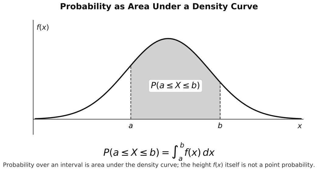How to read this figure. Density height alone is not probability. The shaded probability combines height and interval width as area; the non-normal curve prevents the area rule from being confused with a special property of normal distributions.

Valid Pdf Conditions

A valid pdf must satisfy two conditions.

First,

$$f(x)\ge 0$$

for all values in its domain. Negative density would lead to negative probability over small intervals, which is impossible.

Second,

$${\int }_{\text{all }x}f(x)dx=1.$$

This says the total area under the whole density curve is $1$.

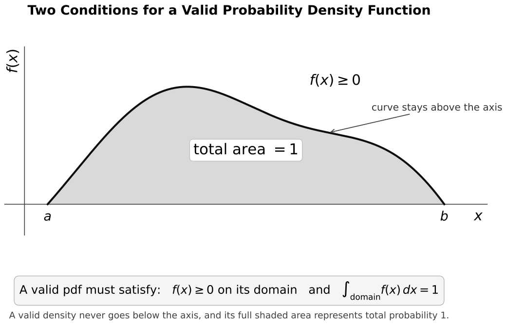How to read this figure. Non-negativity and total area $1$ are simultaneous conditions over the entire support. The condition is on total area, not on every height being at most $1$.

Do not check only whether the formula looks positive. Always check the intended domain. A function may be non-negative on one interval but invalid if the total area is not $1$.

Density Is Not Probability

A density value such as $f(2)$ is not the probability that $X=2$.

The value $f(2)$ is a height. It tells us how concentrated the distribution is near $2$, but it has no interval width by itself. Probability needs area.

This is why a density value may be greater than $1$ without causing a contradiction. A tall, narrow density can still have total area $1$.

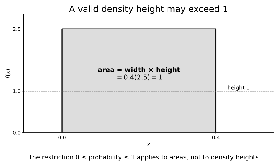
How to read this figure. The rectangle has height $2.5>1$ but width $0.4$, so its total area is $2.5(0.4)=1$. Density is measured per unit of $X$; only probability areas must lie between $0$ and $1$.

The safe reading is:

Height is density. Area is probability.

Exact-Point Probability

For any continuous random variable,

$$P(X=a)=0.$$

This follows directly from the area interpretation:

$$P(X=a)={\int }_a^{a}f(x)dx=0.$$

A single point has zero width. Since probability is area, it contributes zero probability.

This does not mean the value $a$ is impossible in practical language. It means the model gives probability to intervals such as

$$a-0.1<X<a+0.1,$$

not to the infinitely precise point $X=a$.

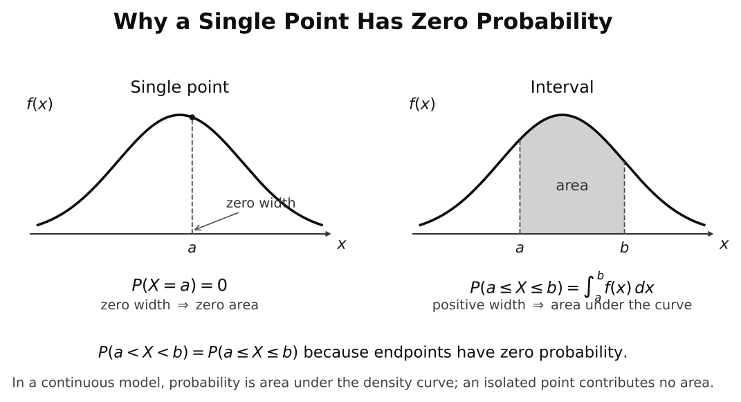How to read this figure. A zero-width point contributes zero area. Therefore open and closed versions of the same finite interval have equal probabilities in this model.

Endpoint Conventions

Because exact-point probabilities are zero, endpoint inclusion does not matter for continuous random variables.

For example,

$$P(X<a)=P(X\le a)$$

and

$$P(a<X<b)=P(a\le X<b)=P(a<X\le b)=P(a\le X\le b).$$

This is different from discrete random variables. In a discrete model, adding or removing a possible value can change the probability. In a continuous model, adding or removing finitely many endpoints does not change area.

Cumulative Distribution Function

The cumulative distribution function, or cdf, is

$$F(x)=P(X\le x).$$

It measures probability accumulated up to $x$.

If the pdf is $f(x)$, then

$$F(x)={\int }_{-\infty }^{x}f(t)dt.$$

If the random variable is defined only from a lower endpoint $c$, this is often written as

$$F(x)={\int }_c^{x}f(t)dt$$

for values of $x$ inside the domain.

The cdf has four universal properties for an absolutely continuous model:

• $F(x)$ is non-decreasing;
• $F(x)$ is continuous;
• $0\le F(x)\le 1$;
• $F(x)\to 0$ as $x\to -\infty$ and $F(x)\to 1$ as $x\to \infty$.

If the support has a finite lower endpoint, $F(x)=0$ at and below the region before probability begins. If it has a finite upper endpoint $b$, then $F(x)=1$ for $x\ge b$.

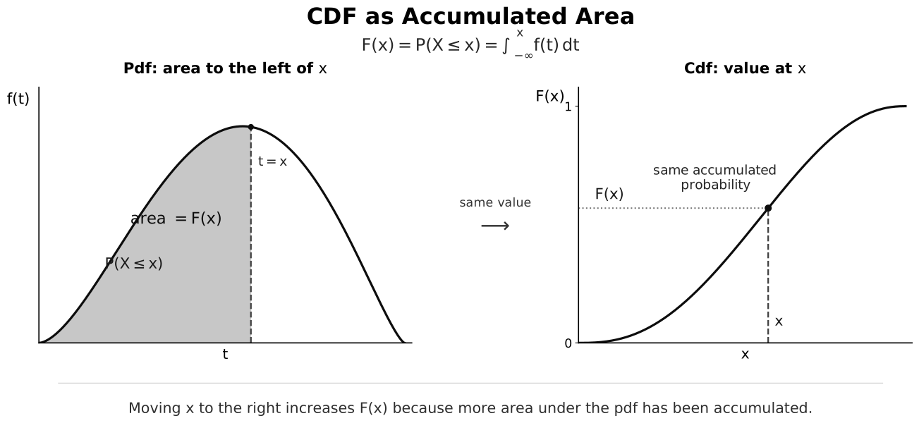How to read this figure. Moving $x$ right accumulates more area, so $F(x)$ cannot decrease. The displayed CDF is matched exactly to the displayed pdf; other pdfs produce other non-decreasing CDF shapes, not necessarily a sigmoid.

Using the CDF for Intervals

The cdf collects probability from the left. Therefore

$$P(a<X<b)=F(b)-F(a).$$

The subtraction removes the area accumulated before $a$, leaving only the area between $a$ and $b$.

Common translations are:

Wording	Probability form
less than $a$	$P(X<a)=F(a)$
at most $a$	$P(X\le a)=F(a)$
more than $a$	$P(X>a)=1-F(a)$
at least $a$	$P(X\ge a)=1-F(a)$
between $a$ and $b$	$F(b)-F(a)$
outside $[a,b]$	$F(a)+[1-F(b)]$

For continuous variables, the endpoint versions are equivalent. The important work is identifying the correct interval.

Worked Example: Constant Density

Let

$$f(x)=\frac{1}{4},0\le x\le 4,$$

and $f(x)=0$ otherwise.

First check that the total area is $1$:

$${\int }_0^4\frac{1}{4}dx=1.$$

So $f$ is a valid pdf.

Now find

$$P(1\le X\le 3).$$

Using area,

$$P(1\le X\le 3)={\int }_1^3\frac{1}{4}dx=\frac{1}{2}.$$

This probability is the area of a rectangle of width $2$ and height $\frac{1}{4}$. It is not the density height $\frac{1}{4}$.

The cdf is

$$F(x)=\{\begin{array}{ll}0,& x<0,\\ \frac{x}{4},& 0\le x\le 4,\\ 1,& x>4.\end{array}$$

Then

$$F(3)-F(1)=\frac{3}{4}-\frac{1}{4}=\frac{1}{2},$$

which matches the area calculation.

Worked Example: Non-Uniform Density

Let

$$f(x)=2x,0\le x\le 1,$$

and $f(x)=0$ otherwise.

This density is not constant. Values near $1$ have greater density than values near $0$, but probability still comes from area, not from height alone.

First check that $f$ is a valid pdf:

$${\int }_0^{1}2xdx=[x^2{]}_0^1=1.$$

To build the cdf, accumulate area from the left:

$$F(x)=\{\begin{array}{ll}0,& x<0,\\ {\int }_0^{x}2tdt=x^2,& 0\le x\le 1,\\ 1,& x>1.\end{array}$$

Now find

$$P(0.3<X<0.8).$$

Using the cdf,

$$P(0.3<X<0.8)=F(0.8)-F(0.3)=0.8^2-0.3^2=\mathrm{0.55.}$$

The same answer comes from the area integral:

$${\int }_{0.3}^{0.8}2xdx=\mathrm{0.55.}$$

Also,

$$P(X=0.5)=0,$$

even though $f(0.5)=1$. The number $1$ is a density height, not the probability of the exact point.

Where the CDF is differentiable,

$$F^{\prime }(x)=f(x).$$

Thus the pdf is the rate at which cumulative probability grows. In this example, $F^{\prime }(x)=2x$ on $(0,1)$, exactly recovering the pdf.

Worked Example: Finding a Normalising Constant

Suppose

$$f(x)=kx(2-x),0\le x\le 2,$$

and $f(x)=0$ otherwise. Since $x(2-x)\ge 0$ on the support, non-negativity will hold once $k>0$. Use total area $1$:

$$1=k{\int }_0^{2}x(2-x)dx=k{\left[x^2-\frac{x^3}{3}\right]}_0^2=\frac{4k}{3}.$$

Hence $k=\frac{3}{4}$. Therefore

$$P(0.5<X<1.5)=\frac{3}{4}{\left[x^2-\frac{x^3}{3}\right]}_{0.5}^{1.5}=\frac{11}{16}.$$

The workflow is: state the support, impose total area $1$, check non-negativity, and only then calculate probabilities.

Quantiles and Inverting the CDF

When the solution is unique, the $p$-quantile $q$ satisfies

$$F(q)=p.$$

For example, a median $m$ satisfies $F(m)=0.5$. Inverse-normal calculator commands apply this same idea to the normal CDF; they return a boundary when a cumulative probability is given.

This example is a useful bridge to the normal distribution. For the normal curve, the pdf is more complicated, so most areas are found with a calculator, but the meaning is the same: interval probability is accumulated area.

Common Pitfalls

Mistake	Correction
Reading $f(a)$ as $P(X=a)$	$f(a)$ is density, not probability.
Forgetting to check total area	A valid pdf must integrate to $1$.
Worrying about open or closed endpoints	Endpoints do not affect continuous probabilities.
Using $F(b)+F(a)$ for an interval	Use $F(b)-F(a)$.
Ignoring the domain	Outside the domain, the density may be $0$ and the cdf may be constant.

Revision Checklist

• Can you explain why probability is area in a continuous model?
• Can you state the two validity conditions for a pdf?
• Can you explain why a density value may exceed $1$?
• Can you explain why $P(X=a)=0$?
• Can you use endpoint equivalence correctly?
• Can you define $F(x)=P(X\le x)$?
• Can you use $F(b)-F(a)$ to find an interval probability?
• Can you build a simple cdf by integrating a pdf over the correct domain?
• Can you interpret $F^{\prime }(x)=f(x)$ where the CDF is differentiable?
• Can you use total area $1$ to determine an unknown density constant?
• Can you interpret a quantile as a solution of $F(q)=p$?
• Can you explain why calculator normal-cdf values are still accumulated areas?